Tutorials

• 1: Bash basics
• 2: Slurm basics
• 3: Apptainer tutorial
• 4: Vim basics
• 5: Python environments
• 6: Multi-GPU training

flowchart TB
    subgraph local["YOUR COMPUTER"]
        L1["Write code, prepare data"]
    end

    subgraph login["LOGIN NODE - daic01.hpc.tudelft.nl"]
        L2["Prepare scripts"]
        L3["Submit jobs (sbatch)"]
        L4["Monitor jobs (squeue)"]
        L5["Transfer data (scp, rsync)"]
        L6["DO NOT run computations here!"]
    end

    subgraph compute["COMPUTE NODES - gpu01...gpu45"]
        C1["Run training scripts"]
        C2["Access GPUs (L40, A40, RTX Pro 6000)"]
        C3["Process large datasets"]
    end

    subgraph storage["STORAGE"]
        S1["/home - 5 MB, config only"]
        S2["~/linuxhome - ~30 GB, personal files"]
        S3["staff-umbrella - Project data"]
    end

    local -->|SSH| login
    login -->|Slurm| compute
    compute --> storage

1 - Bash basics

What you’ll learn

By the end of this tutorial, you’ll be able to:

• Navigate the DAIC filesystem confidently
• Create, copy, move, and delete files and directories
• Redirect command output (stdout/stderr) to files
• Find files and search their contents
• Write simple shell scripts to automate tasks

Time: About 30 minutes

Prerequisites: You should have logged into DAIC at least once.

The scenario

You’re a researcher who just got access to DAIC. You need to:

1. Set up a project directory
2. Organize your files
3. Find things when you forget where you put them
4. Automate repetitive tasks with scripts

Let’s learn the commands you need by actually doing these tasks.

Part 1: Finding your way around

When you log into DAIC, you arrive at your home directory. But where exactly are you, and what’s here?

Where am I?

The pwd command (print working directory) shows your current location:

$ pwd
/home/netid01

You’re in your home directory. On DAIC, this is a small space (5 MB) meant only for configuration files - not for your actual work.

What’s here?

The ls command lists what’s in the current directory:

$ ls
linuxhome

Not much! Let’s see more detail with ls -la:

$ ls -la
total 12
drwxr-xr-x   3 netid01 netid01 4096 Mar 20 09:00 .
drwxr-xr-x 100 root    root    4096 Mar 20 08:00 ..
-rw-r--r--   1 netid01 netid01  220 Mar 20 09:00 .bashrc
lrwxrwxrwx   1 netid01 netid01   45 Mar 20 09:00 linuxhome -> /tudelft.net/staff-homes-linux/n/netid01

Now we see hidden files (starting with .) and details about each file. The linuxhome entry has an arrow - it’s a symbolic link pointing to your larger personal storage.

$ kinit
Password for netid01@TUDELFT.NET:

Moving around

The cd command (change directory) moves you to a different location:

$ cd linuxhome
$ pwd
/home/netid01/linuxhome

Some useful shortcuts:

$ cd ..        # Go up one level
$ cd ~         # Go to home directory
$ cd -         # Go back to previous directory
$ cd           # Also goes to home directory

Exercise 1: Explore the filesystem

Try these commands and observe what happens:

$ cd /tudelft.net/staff-umbrella
$ ls
$ cd ~
$ pwd

Part 2: Understanding DAIC storage

Before we create files, let’s understand where to put them. DAIC has several storage locations:

Rule of thumb:

• Code and small files → linuxhome or umbrella
• Large datasets → umbrella
• Never put large files in /home

Let’s navigate to where you’ll do most of your work:

$ cd /tudelft.net/staff-umbrella
$ ls

You should see one or more project directories. For this tutorial, let’s assume you have access to a project called myproject:

$ cd myproject
$ pwd
/tudelft.net/staff-umbrella/myproject

Part 3: Creating a project structure

Now let’s set up a workspace for a machine learning project.

Creating directories

The mkdir command creates directories:

$ mkdir ml-experiment
$ cd ml-experiment
$ pwd
/tudelft.net/staff-umbrella/myproject/ml-experiment

Create multiple directories at once with -p (which also creates parent directories if needed):

$ mkdir -p data/raw data/processed models results logs
$ ls
data  logs  models  results
$ ls data
processed  raw

We’ve created this structure:

ml-experiment/
├── data/
│   ├── raw/
│   └── processed/
├── models/
├── results/
└── logs/

Creating files

Create a simple file with echo and redirection:

$ echo "# ML Experiment" > README.md
$ cat README.md
# ML Experiment

The > operator writes output to a file, overwriting any existing content.

Output redirection

Every command has two output channels:

• Standard output (stdout) - normal output (file descriptor 1)
• Standard error (stderr) - error messages (file descriptor 2)

By default, both print to your terminal. Redirection lets you send them elsewhere.

Redirect stdout to a file:

$ echo "Hello" > output.txt       # Overwrite file
$ echo "World" >> output.txt      # Append to file
$ cat output.txt
Hello
World

Redirect stderr to a file:

$ ls /nonexistent 2> errors.txt   # Errors go to file
$ cat errors.txt
ls: cannot access '/nonexistent': No such file or directory

Redirect both stdout and stderr:

$ python train.py > output.txt 2>&1    # Both to same file
$ python train.py &> output.txt        # Shorthand (bash 4+)

The 2>&1 syntax means “redirect file descriptor 2 (stderr) to wherever file descriptor 1 (stdout) is going.”

Separate files for stdout and stderr:

$ python train.py > results.txt 2> errors.txt

Discard output entirely:

$ command > /dev/null 2>&1        # Discard everything
$ command 2> /dev/null            # Discard only errors

Exercise 2: Build your own structure

Create a directory structure for a different project:

$ cd /tudelft.net/staff-umbrella/myproject
$ mkdir -p nlp-project/{data,src,notebooks,outputs}
$ ls nlp-project

Then create a README:

$ echo "# NLP Project" > nlp-project/README.md
$ echo "Author: $(whoami)" >> nlp-project/README.md
$ cat nlp-project/README.md

data  notebooks  outputs  src

# NLP Project
Author: <your-netid>

Part 4: Working with files

Let’s create some actual code to work with.

Creating a Python script

We’ll use cat with a “here document” to create a multi-line file:

$ cd /tudelft.net/staff-umbrella/myproject/ml-experiment
$ cat > train.py << 'EOF'
#!/usr/bin/env python3
"""Simple training script."""

import argparse

def main():
    parser = argparse.ArgumentParser()
    parser.add_argument('--epochs', type=int, default=10)
    parser.add_argument('--lr', type=float, default=0.001)
    args = parser.parse_args()

    print(f"Training for {args.epochs} epochs with lr={args.lr}")
    for epoch in range(args.epochs):
        print(f"Epoch {epoch+1}/{args.epochs}")
    print("Done!")

if __name__ == '__main__':
    main()
EOF

Verify the file was created:

$ cat train.py
$ ls -l train.py
-rw-r--r-- 1 netid01 netid01 423 Mar 20 10:35 train.py

Copying files

The cp command copies files:

$ cp train.py train_backup.py
$ ls
data  logs  models  README.md  results  train_backup.py  train.py

Copy entire directories with -r (recursive):

$ cp -r data data_backup
$ ls
data  data_backup  logs  models  README.md  results  train_backup.py  train.py

Moving and renaming

The mv command moves files. It’s also how you rename:

$ mv train_backup.py old_train.py      # Rename
$ mv old_train.py models/              # Move to models directory
$ ls models
old_train.py

Deleting files

The rm command removes files:

$ rm models/old_train.py
$ ls models

Delete directories with -r:

$ rm -r data_backup
$ ls
data  logs  models  README.md  results  train.py

Exercise 3: File operations

Practice by doing the following:

1. Copy train.py to evaluate.py
2. Create a src directory
3. Move both Python files into src
4. Verify with ls src

$ cp train.py evaluate.py
$ mkdir src
$ mv train.py evaluate.py src/
$ ls src
evaluate.py  train.py

evaluate.py  train.py

Part 5: Viewing and editing files

Viewing file contents

Several commands let you view files:

$ cat src/train.py              # Print entire file
$ head -n 5 src/train.py        # First 5 lines
$ tail -n 5 src/train.py        # Last 5 lines
$ less src/train.py             # Scrollable viewer (q to quit)

For log files that are being written, tail -f shows new lines as they appear:

$ tail -f logs/training.log     # Watch live (Ctrl+C to stop)

Counting lines

$ wc -l src/train.py
18 src/train.py

Editing files

For quick edits, use nano (beginner-friendly):

$ nano src/train.py

• Type to insert text
• Ctrl+O to save
• Ctrl+X to exit

For more power, use vim (see our Vim tutorial):

$ vim src/train.py

Part 6: Finding things

As your project grows, you’ll need to find files and search their contents.

Finding files by name

The find command searches for files:

$ find . -name "*.py"
./src/train.py
./src/evaluate.py

The . means “start from current directory”. Common options:

$ find . -name "*.py"                    # Files matching pattern
$ find . -type d -name "data*"           # Directories only
$ find . -type f -mtime -7               # Files modified in last 7 days
$ find . -size +100M                     # Files larger than 100MB

Searching inside files

The grep command searches file contents:

$ grep "epochs" src/train.py
    parser.add_argument('--epochs', type=int, default=10)
    print(f"Training for {args.epochs} epochs with lr={args.lr}")
    for epoch in range(args.epochs):

Search all Python files recursively:

$ grep -r "import" src/
src/train.py:import argparse

Useful options:

$ grep -n "epochs" src/train.py    # Show line numbers
$ grep -i "EPOCH" src/train.py     # Case-insensitive
$ grep -l "import" src/*.py        # Just show filenames

Exercise 4: Find and search

1. Find all files modified in the last day:

   $ find . -mtime -1
   

2. Search for all occurrences of “print” in your Python files:

   $ grep -n "print" src/*.py
   

3. Find all directories named “data”:

   $ find . -type d -name "data"
   

Part 7: Automating with scripts

When you find yourself typing the same commands repeatedly, it’s time to write a script.

Your first script

Create a script that sets up a new experiment:

$ cat > setup_experiment.sh << 'EOF'
#!/bin/bash
# Setup script for new experiments

# Check if experiment name was provided
if [ -z "$1" ]; then
    echo "Usage: ./setup_experiment.sh <experiment_name>"
    exit 1
fi

EXPERIMENT_NAME=$1
BASE_DIR="/tudelft.net/staff-umbrella/myproject"

echo "Creating experiment: $EXPERIMENT_NAME"

# Create directory structure
mkdir -p "$BASE_DIR/$EXPERIMENT_NAME"/{data,models,results,logs}

# Create a README
cat > "$BASE_DIR/$EXPERIMENT_NAME/README.md" << README
# $EXPERIMENT_NAME

Created: $(date)
Author: $(whoami)

## Description
TODO: Add description

## Results
TODO: Add results
README

echo "Done! Experiment created at $BASE_DIR/$EXPERIMENT_NAME"
ls -la "$BASE_DIR/$EXPERIMENT_NAME"
EOF

Make it executable

Before you can run a script, you need to make it executable:

$ chmod +x setup_experiment.sh
$ ls -l setup_experiment.sh
-rwxr-xr-x 1 netid01 netid01 612 Mar 20 11:00 setup_experiment.sh

The x in the permissions means “executable”.

Run the script

$ ./setup_experiment.sh bert-finetuning
Creating experiment: bert-finetuning
Done! Experiment created at /tudelft.net/staff-umbrella/myproject/bert-finetuning
total 4
drwxr-xr-x 2 netid01 netid01 4096 Mar 20 11:00 data
drwxr-xr-x 2 netid01 netid01 4096 Mar 20 11:00 logs
drwxr-xr-x 2 netid01 netid01 4096 Mar 20 11:00 models
-rw-r--r-- 1 netid01 netid01  142 Mar 20 11:00 README.md
drwxr-xr-x 2 netid01 netid01 4096 Mar 20 11:00 results

Script building blocks

Here are patterns you’ll use often:

Variables:

NAME="experiment1"
echo "Working on $NAME"

Conditionals:

if [ -f "data.csv" ]; then
    echo "Data file exists"
else
    echo "Data file not found!"
    exit 1
fi

Loops:

for file in data/*.csv; do
    echo "Processing $file"
    python process.py "$file"
done

Command substitution:

TODAY=$(date +%Y-%m-%d)
echo "Running on $TODAY"

Exercise 5: Write a cleanup script

Create a script that removes old log files:

$ cat > cleanup_logs.sh << 'EOF'
#!/bin/bash
# Remove log files older than 7 days

LOG_DIR="${1:-.}"  # Use first argument, or current directory

echo "Cleaning logs in $LOG_DIR"

# Find and remove old logs
find "$LOG_DIR" -name "*.log" -mtime +7 -exec rm -v {} \;

echo "Done!"
EOF

$ chmod +x cleanup_logs.sh
$ ./cleanup_logs.sh logs/

$ ls -l cleanup_logs.sh
-rwxr-xr-x 1 netid01 netid01 ... cleanup_logs.sh

Part 8: Useful shortcuts and tips

Tab completion

Press Tab to autocomplete:

• Filenames
• Directory names
• Commands

$ cd /tudelft.net/staff-umb<TAB>
$ cd /tudelft.net/staff-umbrella/

Command history

$ history              # Show recent commands
$ !42                  # Run command number 42
$ !!                   # Run the last command
$ !grep                # Run the last command starting with "grep"

Press Ctrl+R to search history interactively.

Keyboard shortcuts

Aliases

Create shortcuts for common commands. Add to ~/.bashrc:

alias ll='ls -lah'
alias umbrella='cd /tudelft.net/staff-umbrella/myproject'
alias jobs='squeue -u $USER'

Then reload:

$ source ~/.bashrc
$ umbrella    # Now this works!

Summary

You’ve learned to:

What’s next?

Now that you’re comfortable with the command line:

1. Data Transfer - Move data to and from DAIC
2. Slurm Tutorial - Learn to submit jobs to the cluster
3. Vim Tutorial - Edit files more efficiently
4. Shell Setup - Configure your environment

Quick reference

For more advanced shell customization, see Shell Setup.

2 - Slurm basics

What you’ll learn

By the end of this tutorial, you’ll be able to:

• Submit batch jobs that run on compute nodes
• Request CPUs, memory, and GPUs for your jobs
• Monitor job status and troubleshoot failures
• Use interactive sessions for testing
• Run parameter sweeps with job arrays

Time: About 45 minutes

Prerequisites: Complete the Bash Basics tutorial first, or be comfortable with Linux command line.

What is Slurm?

When you log into DAIC, you land on a login node. This is a shared computer where users prepare their work - but you shouldn’t run computations here. The actual computing happens on compute nodes, powerful machines with GPUs and lots of memory.

Slurm is the traffic controller that manages these compute nodes. When you want to run a computation, you don’t run it directly - you ask Slurm to run it for you. Slurm finds available resources, starts your job, and makes sure it doesn’t interfere with other users’ jobs.

Think of it like a restaurant: you don’t walk into the kitchen and cook your own food. You submit an order (your job), and the kitchen (Slurm) prepares it when they have capacity.

Why can’t I just run my code?

You might wonder: “Why can’t I just type python train.py and let it run?”

On a personal computer, that works fine. But DAIC is shared by hundreds of researchers, each wanting to use expensive GPUs. Without a scheduler:

• Everyone would fight over the same resources
• Your job might get killed when someone else starts theirs
• GPUs would sit idle when no one happens to be logged in
• There would be no fairness - whoever types fastest wins

Slurm solves these problems by:

• Queueing jobs and running them in order
• Guaranteeing that your job gets the resources you requested
• Ensuring fair access based on policies
• Maximizing utilization of expensive hardware

The two ways to run jobs

Batch jobs: submit and walk away

Most of the time, you’ll use batch jobs. You write a script that describes what you want to run, submit it, and Slurm runs it whenever resources are available. You don’t need to stay logged in - you can submit at 5pm, go home, and check results the next morning.

$ sbatch my_job.sh
Submitted batch job 12345

Your job enters a queue. When resources become available, Slurm runs it. Output goes to a file you can read later.

Interactive jobs: real-time access

Sometimes you need to work interactively - debugging, testing, or exploring data. For this, you request an interactive job. Slurm allocates resources, and you get a shell on a compute node.

$ salloc --account=<your-account> --partition=all --time=1:00:00 --gres=gpu:1
salloc: Granted job allocation 12346
$ srun nvidia-smi
$ srun python -c "import torch; print(torch.cuda.is_available())"
True

Interactive jobs are great for testing but expensive - you’re reserving resources the whole time, even if you’re just thinking. Use batch jobs for actual computations.

Your first batch job

Let’s walk through creating and submitting a batch job step by step.

Step 1: Create a Python script

First, create a simple script to run. This one just prints some information:

$ cd /tudelft.net/staff-umbrella/<project>
$ vim hello.py

import socket
import os

print(f"Hello from {socket.gethostname()}")
print(f"Job ID: {os.environ.get('SLURM_JOB_ID', 'not in slurm')}")
print(f"CPUs allocated: {os.environ.get('SLURM_CPUS_PER_TASK', 'unknown')}")

Step 2: Create a batch script

Now create the Slurm script that will run your Python code:

$ vim hello_job.sh

#!/bin/bash
#SBATCH --account=<your-account>
#SBATCH --partition=all
#SBATCH --time=0:10:00
#SBATCH --ntasks=1
#SBATCH --cpus-per-task=1
#SBATCH --mem=1G
#SBATCH --output=hello_%j.out

echo "Job started at $(date)"

srun python hello.py

echo "Job finished at $(date)"

Let’s understand each line:

Step 3: Find your account

Before submitting, you need to know your account name:

$ sacctmgr show associations user=$USER format=Account -P
Account
ewi-insy-reit

Replace <your-account> in your script with this value (e.g., ewi-insy-reit).

Step 4: Submit the job

$ sbatch hello_job.sh
Submitted batch job 12345

The number 12345 is your job ID. You’ll use this to track your job.

Step 5: Check job status

$ squeue -u $USER
  JOBID PARTITION     NAME     USER ST       TIME  NODES NODELIST(REASON)
  12345       all hello_jo  netid01 PD       0:00      1 (Priority)

The ST column shows the status:

• PD = Pending - waiting in queue
• R = Running
• CG = Completing - wrapping up

The REASON column tells you why a job is pending:

• Priority = other jobs are ahead of you in the queue
• Resources = waiting for nodes to become free
• QOSMaxJobsPerUserLimit = you’ve hit your job limit

Step 6: Check the output

Once the job completes, read the output file:

$ cat hello_12345.out
Job started at Fri Mar 20 10:15:32 CET 2026
Hello from gpu23.ethernet.tudhpc
Job ID: 12345
CPUs allocated: 1
Job finished at Fri Mar 20 10:15:33 CET 2026

Your code ran on gpu23, not on the login node. Slurm handled everything.

Understanding resource requests

The most confusing part of Slurm is figuring out what resources to request. Request too little and your job crashes; request too much and you wait longer in the queue.

Time (--time)

How long your job will run. Format: D-HH:MM:SS or HH:MM:SS

#SBATCH --time=0:30:00      # 30 minutes
#SBATCH --time=4:00:00      # 4 hours
#SBATCH --time=1-00:00:00   # 1 day
#SBATCH --time=7-00:00:00   # 7 days (maximum on DAIC)

Important: If your job exceeds this time, Slurm kills it. But requesting more time means waiting longer in the queue. Start with a generous estimate, then use seff on completed jobs to tune it.

Memory (--mem)

How much RAM your job needs.

#SBATCH --mem=4G      # 4 gigabytes
#SBATCH --mem=32G     # 32 gigabytes
#SBATCH --mem=128G    # 128 gigabytes

If your job exceeds this limit, Slurm kills it with an “out of memory” error. Check your code’s actual memory usage with seff after a successful run.

CPUs (--cpus-per-task)

How many CPU cores your job needs.

#SBATCH --cpus-per-task=1    # Single-threaded code
#SBATCH --cpus-per-task=4    # Code that uses 4 threads
#SBATCH --cpus-per-task=16   # Heavily parallel CPU code

Match this to what your code actually uses:

• Simple Python scripts: 1 CPU
• PyTorch with DataLoader workers: workers + 1 (e.g., 4 workers = 5 CPUs)
• NumPy/Pandas with parallelism: however many threads you configure

GPUs (--gres)

Request GPUs with the --gres (generic resources) option:

#SBATCH --gres=gpu:1    # One GPU (any type)
#SBATCH --gres=gpu:2    # Two GPUs
#SBATCH --gres=gpu:l40:1   # Specifically an L40 GPU
#SBATCH --gres=gpu:a40:2   # Two A40 GPUs

Available GPU types on DAIC include L40, A40, and RTX Pro 6000. Request specific types only if your code requires it - being flexible gets you through the queue faster.

Running GPU jobs

Most deep learning jobs need GPUs. Here’s a complete example:

The Python training script

# train.py
import torch
import torch.nn as nn

# Check GPU availability
device = torch.device('cuda' if torch.cuda.is_available() else 'cpu')
print(f"Using device: {device}")

if torch.cuda.is_available():
    print(f"GPU: {torch.cuda.get_device_name(0)}")
    print(f"Memory: {torch.cuda.get_device_properties(0).total_memory / 1e9:.1f} GB")

# Simple training loop
model = nn.Linear(1000, 100).to(device)
optimizer = torch.optim.Adam(model.parameters())

for epoch in range(100):
    x = torch.randn(64, 1000, device=device)
    y = model(x)
    loss = y.sum()
    optimizer.zero_grad()
    loss.backward()
    optimizer.step()

    if epoch % 10 == 0:
        print(f"Epoch {epoch}, loss: {loss.item():.4f}")

print("Training complete!")

The batch script

#!/bin/bash
#SBATCH --account=<your-account>
#SBATCH --partition=all
#SBATCH --time=1:00:00
#SBATCH --ntasks=1
#SBATCH --cpus-per-task=4
#SBATCH --mem=16G
#SBATCH --gres=gpu:1
#SBATCH --output=train_%j.out

# Clean environment and load required modules
module purge
module load 2025/gpu cuda/12.9

# Print job info for debugging
echo "Job ID: $SLURM_JOB_ID"
echo "Running on: $(hostname)"
echo "GPUs: $CUDA_VISIBLE_DEVICES"
echo "Start time: $(date)"

# Run training
srun python train.py

echo "End time: $(date)"

Understanding the module system

DAIC uses an environment modules system to manage software. Instead of having every version of every library available at once (which would cause conflicts), software is organized into modules that you load when needed.

The module commands set up your software environment:

module purge            # Clear any previously loaded modules
module load 2025/gpu    # Load the 2025 GPU software stack
module load cuda/12.9   # Load CUDA 12.9

Why use modules?

• Version control: Run module load python/3.11 today, python/3.12 tomorrow
• Avoid conflicts: Different projects can use different library versions
• Clean environment: module purge gives you a fresh start

Common module commands:

For a complete guide, see Loading Software.

Submit and monitor

$ sbatch train_job.sh
Submitted batch job 12350

$ squeue -u $USER
  JOBID PARTITION     NAME     USER ST       TIME  NODES NODELIST(REASON)
  12350       all train_jo  netid01  R       0:45      1 gpu15

$ tail -f train_12350.out
Job ID: 12350
Running on: gpu15.ethernet.tudhpc
GPUs: 0
Start time: Fri Mar 20 11:00:00 CET 2026
Using device: cuda
GPU: NVIDIA L40
Memory: 45.0 GB
Epoch 0, loss: 156.7823
Epoch 10, loss: 89.3421
...

The tail -f command shows output in real-time as your job runs.

Interactive jobs for testing

Before submitting a long batch job, test your code interactively:

Request an interactive session

$ salloc --account=<your-account> --partition=all --time=1:00:00 --cpus-per-task=4 --mem=8G --gres=gpu:1
salloc: Pending job allocation 12351
salloc: job 12351 queued and waiting for resources
salloc: job 12351 has been allocated resources
salloc: Granted job allocation 12351

You now have resources reserved. But you’re still on the login node - you need srun to actually use the compute node:

Run commands on the compute node

$ srun hostname
gpu15.ethernet.tudhpc

$ srun nvidia-smi
+-----------------------------------------------------------------------------+
| NVIDIA-SMI 550.54.15    Driver Version: 550.54.15    CUDA Version: 12.9     |
|-------------------------------+----------------------+----------------------+
| GPU  Name        Persistence-M| Bus-Id        Disp.A | Volatile Uncorr. ECC |
| Fan  Temp  Perf  Pwr:Usage/Cap|         Memory-Usage | GPU-Util  Compute M. |
|===============================+======================+======================|
|   0  NVIDIA L40          On   | 00000000:41:00.0 Off |                    0 |
| N/A   30C    P8    22W / 300W |      0MiB / 46068MiB |      0%      Default |
+-------------------------------+----------------------+----------------------+

$ srun python train.py
Using device: cuda
...

Start an interactive shell on the compute node

For more extended testing, start a shell on the compute node:

$ srun --pty bash
$ hostname
gpu15.ethernet.tudhpc
$ python train.py
...
$ exit

Don’t forget to release resources

When done testing, release your allocation:

$ exit
salloc: Relinquishing job allocation 12351

If you forget, you’ll hold resources for the full time you requested, even if you’re not using them. This isn’t fair to other users.

Job arrays: running many similar jobs

Often you need to run the same code with different parameters - different random seeds, different hyperparameters, or different data splits. Job arrays make this easy.

The problem

You want to run your experiment with seeds 1 through 10. You could submit 10 separate jobs:

$ sbatch --export=SEED=1 experiment.sh
$ sbatch --export=SEED=2 experiment.sh
$ sbatch --export=SEED=3 experiment.sh
... # tedious!

The solution: job arrays

Instead, use a single job array:

#!/bin/bash
#SBATCH --account=<your-account>
#SBATCH --partition=all
#SBATCH --time=2:00:00
#SBATCH --cpus-per-task=4
#SBATCH --mem=16G
#SBATCH --gres=gpu:1
#SBATCH --array=1-10
#SBATCH --output=experiment_%A_%a.out

# %A = array job ID, %a = array task ID
echo "Array job ID: $SLURM_ARRAY_JOB_ID"
echo "Array task ID: $SLURM_ARRAY_TASK_ID"

srun python experiment.py --seed $SLURM_ARRAY_TASK_ID

Submit once, get 10 jobs:

$ sbatch experiment_array.sh
Submitted batch job 12360

$ squeue -u $USER
  JOBID PARTITION     NAME     USER ST       TIME  NODES NODELIST(REASON)
12360_1       all experime  netid01  R       0:30      1 gpu01
12360_2       all experime  netid01  R       0:30      1 gpu02
12360_3       all experime  netid01  R       0:30      1 gpu03
12360_4       all experime  netid01 PD       0:00      1 (Resources)
...

Array variations

#SBATCH --array=1-100        # Tasks 1 through 100
#SBATCH --array=0-9          # Tasks 0 through 9
#SBATCH --array=1,3,5,7      # Just these specific tasks
#SBATCH --array=1-100%10     # 1-100, but max 10 running at once

The %10 syntax limits concurrent tasks, useful if you don’t want to flood the queue.

Using array indices creatively

Your Python code can use $SLURM_ARRAY_TASK_ID for more than just seeds:

import os
import json

task_id = int(os.environ.get('SLURM_ARRAY_TASK_ID', 0))

# Load hyperparameter configurations
with open('configs.json') as f:
    configs = json.load(f)

config = configs[task_id]
print(f"Running with config: {config}")

Where configs.json contains:

[
  {"lr": 0.001, "batch_size": 32},
  {"lr": 0.001, "batch_size": 64},
  {"lr": 0.01, "batch_size": 32},
  {"lr": 0.01, "batch_size": 64}
]

Job dependencies: workflows

Sometimes jobs must run in a specific order. Job dependencies let you express this.

Run after another job succeeds

$ sbatch preprocess.sh
Submitted batch job 12370

$ sbatch --dependency=afterok:12370 train.sh
Submitted batch job 12371

Job 12371 won’t start until job 12370 completes successfully. If 12370 fails, 12371 never runs.

Dependency types

Complex workflows

Chain multiple dependencies:

$ sbatch download_data.sh
Submitted batch job 12380

$ sbatch --dependency=afterok:12380 preprocess.sh
Submitted batch job 12381

$ sbatch --dependency=afterok:12381 train.sh
Submitted batch job 12382

$ sbatch --dependency=afterok:12382 evaluate.sh
Submitted batch job 12383

Or depend on multiple jobs:

$ sbatch train_model_a.sh
Submitted batch job 12390

$ sbatch train_model_b.sh
Submitted batch job 12391

$ sbatch --dependency=afterok:12390:12391 ensemble.sh
Submitted batch job 12392

Job 12392 waits for both 12390 and 12391 to complete.

Checking job history and efficiency

View past jobs

$ sacct -u $USER --starttime=2026-03-01
JobID           JobName  Partition    Account  AllocCPUS      State ExitCode
------------ ---------- ---------- ---------- ---------- ---------- --------
12340          training        all  ewi-insy          8  COMPLETED      0:0
12341            failed        all  ewi-insy          4     FAILED      1:0
12342          training        all  ewi-insy          8    TIMEOUT      0:0

Exit codes:

• 0:0 = success
• 1:0 = your code exited with error
• 0:9 = killed by signal 9 (often out of memory)
• TIMEOUT = exceeded time limit

Check efficiency

The seff command shows how well you used the resources you requested:

$ seff 12340
Job ID: 12340
Cluster: daic
State: COMPLETED
Nodes: 1
Cores per node: 8
CPU Utilized: 06:30:15
CPU Efficiency: 81.3% of 08:00:00 core-walltime
Job Wall-clock time: 01:00:00
Memory Utilized: 24.5 GB
Memory Efficiency: 76.6% of 32.0 GB

This job used 81% of allocated CPU and 77% of allocated memory - reasonable efficiency. If you see numbers below 50%, you’re requesting more than you need.

Adjusting based on efficiency

If seff shows:

• Low CPU efficiency: Reduce --cpus-per-task
• Low memory efficiency: Reduce --mem
• Very high efficiency (>95%): Consider requesting slightly more headroom

Troubleshooting

Job stuck in pending

Check why with squeue:

$ squeue -u $USER
  JOBID PARTITION     NAME     USER ST       TIME  NODES NODELIST(REASON)
  12345       all training  netid01 PD       0:00      1 (Resources)

Common reasons:

• Priority - Other jobs are ahead of you. Wait, or request fewer resources.
• Resources - Not enough free nodes. Wait, or request fewer resources.
• QOSMaxJobsPerUserLimit - You’ve hit your concurrent job limit. Wait for some to finish.
• AssocMaxJobsLimit - Your account has hit its limit.

Job killed immediately

Check the output file for errors. Common issues:

Out of memory:

slurmstepd: error: Detected 1 oom-kill event(s) in step 12345.0

Solution: Increase --mem

Time limit:

slurmstepd: error: *** JOB 12345 ON gpu01 CANCELLED AT 2026-03-20T12:00:00 DUE TO TIME LIMIT ***

Solution: Increase --time or add checkpointing to your code

Module not found:

ModuleNotFoundError: No module named 'torch'

Solution: Add module load commands to your script

Can’t find GPUs

Your code can’t see GPUs even though you requested them:

torch.cuda.is_available()  # Returns False

Common causes:

1. Forgot --gres=gpu:1 in your script
2. Running on login node instead of through srun
3. Missing module load cuda
4. CUDA version mismatch

Best practices

1. Test before submitting long jobs

$ salloc --time=0:30:00 --gres=gpu:1 ...
$ srun python train.py --max-epochs 1  # Quick test
$ exit
$ sbatch full_training.sh  # Now submit the real job

2. Request only what you need

Larger requests wait longer in the queue. Start small and increase if needed.

3. Use meaningful job names

#SBATCH --job-name=bert-finetune-lr001

Makes squeue output much more readable.

4. Save checkpoints

For long jobs, save state periodically so you can resume if killed:

# Save checkpoint every epoch
torch.save({
    'epoch': epoch,
    'model_state_dict': model.state_dict(),
    'optimizer_state_dict': optimizer.state_dict(),
}, f'checkpoint_epoch_{epoch}.pt')

5. Use job arrays instead of many scripts

One job array is easier to manage than 100 separate submissions.

6. Check efficiency and tune

After your first successful run, check seff and adjust requests.

Quick reference

Submit and monitor

Information

Common sbatch options

Summary

You’ve learned:

Exercises

Try these on your own to solidify your understanding:

Exercise 1: Basic job submission

Create and submit a job that prints your username, hostname, and current date. Check the output.

netid01
gpu15.ethernet.tudhpc
Fri Mar 20 10:30:00 CET 2026

Exercise 2: GPU job

Modify the basic job to request a GPU. Add nvidia-smi to verify the GPU is available.

+-----------------------------------------------------------------------------+
| NVIDIA-SMI ...    Driver Version: ...    CUDA Version: ...                  |
|-------------------------------+----------------------+----------------------+
| GPU  Name        ...

Exercise 3: Resource tuning

Submit a job, then use seff to check its efficiency. Was your resource request appropriate?

CPU Efficiency: 70-95%
Memory Efficiency: 50-90%

Exercise 4: Job array

Create a job array that runs 5 tasks. Each task should print its array task ID.

$ cat job_*_1.out
Task ID: 1
$ cat job_*_5.out
Task ID: 5

Exercise 5: Dependencies

Submit two jobs where the second depends on the first completing successfully.

  JOBID PARTITION     NAME     USER ST  REASON
  12346       all   second  netid01 PD  (Dependency)
  12345       all    first  netid01  R

Next steps

• Apptainer Tutorial - Package your environment in containers
• Vim Tutorial - Edit files efficiently on the cluster
• Modules - Load pre-installed software

3 - Apptainer tutorial

What you’ll learn

• Understand why containers are useful for HPC workloads
• Pull prebuilt images from Docker Hub and NVIDIA NGC
• Build custom container images from definition files
• Run containerized applications on DAIC with GPU support
• Manage bind mounts and cache directories

Prerequisites: Slurm Basics (submitting jobs, requesting GPUs)

Time: 45 minutes

What and Why containerization?

Containerization packages your software, libraries, and dependencies into a single portable unit: a container. This makes your application behave the same way everywhere: on your laptop, in the cloud, or on DAIC. This means:

• Consistency: The application runs the same way regardless of where it’s executed. You can develop on one machine, test on another, and deploy on a cluster without worrying about dependency differences.
• Isolation: Each container is independent from others, preventing conflicts and enhancing security and reliability.
• Portability: Containers can run on different systems without modification, simplifying movement between servers, clusters, or clouds.
• Efficiency: Containers share the host system’s resources like the operating system, making them lightweight and fast to start compared to virtual machines.

On DAIC specifically, users often encounter issues with limited home directory space or Windows-based /tudelft.net mounts (see Storage), which can complicate the use of conda/mamba and/or pip. Containers offer a solution by encapsulating all software and dependencies in a self-contained environment. You can, for instance, store containers on staff-umbrella with all required dependencies, including those installed via pip, and run them reliably and reproducibly without being limited by home directory size or mount compatibility.

Containerization on DAIC: Apptainer

DAIC supports Apptainer (formerly known as Singularity), an open-source container platform designed for high-performance computing environments. Apptainer runs container images securely on shared clusters and allows you to use Docker images directly, without needing Docker itself.

A typical Apptainer workflow revolves around three key components:

Because Apptainer integrates well with Slurm, containers can be launched directly within batch jobs or interactive sessions on DAIC.
The following sections show how to obtain, build, and run images.

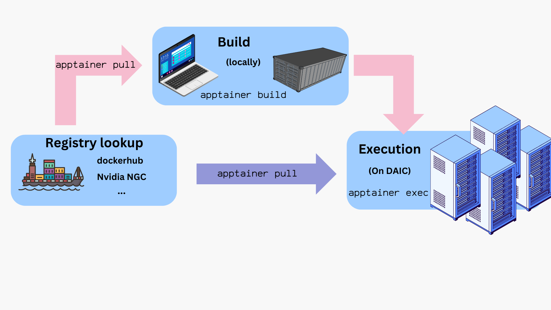
Workflow overview

The typical lifecycle for containers on DAIC is:

1. Build the image locally from a .def file.
2. Transfer or pull the resulting .sif file onto DAIC.
3. Test interactively using salloc to get a compute node.
4. Run in a batch job with sbatch or srun using apptainer exec or apptainer run.
5. Provision bind mounts, GPU flags, and cache locations as needed.
6. Clean up and manage storage (e.g., APPTAINER_CACHEDIR).

How to run commands/programs inside a container?

Once you have a container image (e.g., myimage.sif), you can launch it in different ways depending on how you want to interact with it:

where:

• <image> is the path to a container image, typically, a *.sif file.

Tips:

• Use shell for exploration or debugging inside the container.
• Use exec or run for automation, workflows, or Slurm batch jobs.
• Add -C or -c to isolate the container filesystem (see Exposing host directories).

$ hostname
daic01.hpc.tudelft.nl

$ salloc --account=<your-account> --partition=all --gres=gpu:1 --mem=8G --time=01:00:00
salloc: Granted job allocation 12345

$ srun apptainer exec --nv myimage.sif python script.py

How to get container files?

You can obtain container images in two main ways:

1. Pull prebuilt images by pulling from a container registry/repository (see Using prebuilt images).
2. Build your own image locally using a definition file (*.def), then transfer the resulting .sif file to DAIC (see Building images).

1. Using prebuilt images

Apptainer allows pulling and using images directly from repositories like DockerHub, BioContainers, NVIDIA GPU Cloud (NGC), and others.

Example: Pulling from DockerHub

$ mkdir ~/containers && cd ~/containers

$ apptainer pull docker://ubuntu:latest
INFO:    Converting OCI blobs to SIF format
INFO:    Starting build...
Getting image source signatures
Copying blob 837dd4791cdc done
Copying config 1f6ddc1b25 done
Writing manifest to image destination
...
INFO:    Creating SIF file...

Now, to check the obtained image file:

$ ls
ubuntu_latest.sif

$ apptainer exec ubuntu_latest.sif cat /etc/os-release
PRETTY_NAME="Ubuntu 22.04.2 LTS"
NAME="Ubuntu"
VERSION_ID="22.04"
...

$ ls /.apptainer.d/
ls: cannot access /.apptainer.d/: No such file or directory

$ apptainer shell ubuntu_latest.sif
Apptainer> hostname
daic01.hpc.tudelft.nl
Apptainer> ls /.apptainer.d/
Apptainer  actions  env  labels.json  libs  runscript  startscript
Apptainer> exit

Notes:

• Inside the container, the command prompt changes to Apptainer>
• The container inherits your environment (e.g., $HOME, hostname) but has its own internal filesystem (e.g. /.apptainer.d)

$ apptainer shell -C ubuntu_latest.sif

Example: Pulling from NVIDIA GPU cloud (NGC)

NGC provides pre-built images for GPU accelerated applications. These images are large, so download them locally on your machine and then transfer to DAIC. To install Apptainer locally, follow the official Installing Apptainer instructions.

export APPTAINER_CACHEDIR=/tudelft.net/staff-umbrella/<project>/apptainer/cache

On your local machine:

$ apptainer pull docker://nvcr.io/nvidia/pytorch:24.01-py3
$ scp pytorch_24.01-py3.sif daic01.hpc.tudelft.nl:/tudelft.net/staff-umbrella/<project>/apptainer

Test the image on DAIC:

$ cd /tudelft.net/staff-umbrella/<project>/apptainer

$ salloc --account=<your-account> --partition=all --gres=gpu:1 --time=00:10:00
salloc: Granted job allocation 12345

$ srun apptainer shell -C --nv pytorch_24.01-py3.sif
Apptainer> python -c "import torch; print(torch.cuda.is_available())"
True

2. Building images

If you prefer (or need) a custom container image, you can build one from a definition file (*.def), that specifies your dependencies and setup steps.

On DAIC, you can build images directly if your current directory allows writes and sufficient quota (e.g., under staff-umbrella).
For large or complex builds, it can be more convenient to build locally on your workstation and then transfer the resulting .sif file to DAIC.

$ apptainer build myimage.sif myimage.def

Example: CUDA-enabled container

An example definion file, cuda_based.def, for a cuda-enabled container may look as follows:

# Header
Bootstrap: docker
From: nvidia/cuda:12.1.1-devel-ubuntu22.04

# (Optional) Sections/ data blobs
%post
    apt-get update # update system
    apt-get install -y git   # install git
    git clone https://github.com/NVIDIA/cuda-samples.git  # clone target repository
    cd cuda-samples
    git fetch origin --tags && git checkout v12.1 # fetch certain repository version
    cd Samples/1_Utilities/deviceQuery && make # install certain tool

%runscript
    /cuda-samples/Samples/1_Utilities/deviceQuery/deviceQuery  

where:

• The header, specifies the source (eg, Bootstrap: docker) and the base image (From: nvidia/cuda:12.1.1-devel-ubuntu22.04). Here, the container builds on Ubuntu 22.04 with CUDA 12.1 pre-installed.
• The rest of the file are optional data blobs or sections. In this example, the following blobs are used:
  • %post: the steps to download, configure and install needed custom software and libraries on the base image. In this example, the steps install git, clone a repo, and install a package via make
  • %runscript: the entry point to the container with the apptainer run command. In this example, the deviceQuery is executed once the container is run.
  • Other blobs may be present in the def file. See Definition files documentation for more details and examples.

Build this image locally and transfer it to DAIC:

$ apptainer build cuda_based_image.sif cuda_based.def
INFO:    Starting build...
Getting image source signatures
...
INFO:    Adding runscript
INFO:    Creating SIF file...
INFO:    Build complete: cuda_based_image.sif

$ scp cuda_based_image.sif daic01.hpc.tudelft.nl:/tudelft.net/staff-umbrella/<project>/apptainer

On DAIC, test the image:

$ cd /tudelft.net/staff-umbrella/<project>/apptainer

$ salloc --account=<your-account> --partition=all --cpus-per-task=2 --mem=1G --gres=gpu:1 --time=00:10:00
salloc: Granted job allocation 12345

$ srun apptainer run --nv -C cuda_based_image.sif
/cuda-samples/Samples/1_Utilities/deviceQuery/deviceQuery Starting...

 CUDA Device Query (Runtime API) version (CUDART static linking)

Detected 1 CUDA Capable device(s)

Device 0: "NVIDIA L40"
  CUDA Driver Version / Runtime Version          12.9 / 12.1
  CUDA Capability Major/Minor version number:    8.9
  Total amount of global memory:                 46068 MBytes
  ...
deviceQuery, CUDA Driver = CUDART, CUDA Driver Version = 12.9, CUDA Runtime Version = 12.1, NumDevs = 1
Result = PASS

$ apptainer shell --nv -C cuda_based_image.sif

Example: Extending existing images

During software development, it is common to incrementally build code and go through many iterations of debugging and testing. To save time, you can base a new image on an existing one using the Bootstrap: localimage and From:<path/to/local/image> header. This avoids re-installing the same dependencies with every iteration.

As an example, assume it is desirable to develop some code on the basis of the cuda_based.sif image created in the Example: CUDA-enabled container. Building from the original cuda_based.def file can take ~ 4 minutes. However, if the *.sif file is already available, building on top of it, via a dev_on_cuda_based.def file as below, takes ~ 2 minutes. This is already a time saving factor of 2.

# Header
Bootstrap: localimage
From: cuda_based.sif

# (Optional) Sections/ data blobs
%runscript
    echo "Arguments received: $*"
    exec echo "$@"

Now, build and test:

$ apptainer build dev_image.sif dev_on_cuda_based.def
INFO:    Starting build...
INFO:    Verifying bootstrap image cuda_based.sif
INFO:    Adding runscript
INFO:    Creating SIF file...
INFO:    Build complete: dev_image.sif

$ apptainer run dev_image.sif "hello world"
Arguments received: hello world
hello world

$ apptainer shell dev_image.sif
Apptainer> ls /cuda-samples/Samples/1_Utilities/deviceQuery/deviceQuery
/cuda-samples/Samples/1_Utilities/deviceQuery/deviceQuery

Apptainer> cat /.apptainer.d/bootstrap_history/Apptainer0
bootstrap: docker
from: nvidia/cuda:12.1.1-devel-ubuntu22.04
...

As can be seen in this example, the new def file not only preserves the dependencies of the original image, but it also preserves a complete history of all build processes while giving flexible environment that can be customized as need arises.

Example: Deploying conda and pip in a container

There might be situations where you have a certain conda environment in your local machine that you need to set up in DAIC to commence your analysis. In such cases, deploying your conda environment in a container and sending this container to DAIC does the job for you.

As an example, let’s create a simple demo environment, environment.yml in our local machine,

name: apptainer
channels:
  - conda-forge
  - defaults
dependencies:
  - python=3.9
  - matplotlib
  - pip
  - pip:
    - -r requirements.txt

And everything that should be installed with pip in requirement.txt file:

--extra-index-url https://download.pytorch.org/whl/cu123
torch
annoy

Now, it is time to create the container definition file Apptainer.def. One option is to base the image on condaforge/miniforge, which is a minimal Ubuntu installation with conda preinstalled at /opt/conda:

Bootstrap: docker
From: condaforge/miniforge3:latest

%files
    environment.yml /environment.yml
    requirements.txt /requirements.txt

%post
    # Update and install necessary packages
    apt-get update && apt-get install -y tree time vim ncdu speedtest-cli build-essential

    # Create a new Conda environment using the environment files.
    mamba env create --quiet --file /environment.yml
    
    # Clean up
    apt-get clean && rm -rf /var/lib/apt/lists/*
    mamba clean --all -y

    # Now add the script to activate the Conda environment
    echo '. "/opt/conda/etc/profile.d/conda.sh"' >> $APPTAINER_ENVIRONMENT
    echo 'conda activate apptainer' >> $APPTAINER_ENVIRONMENT

Now, build and check the image:

$ apptainer build demo-env-image.sif Apptainer.def
INFO:    Starting build...
Getting image source signatures
...
INFO:    Creating SIF file...
INFO:    Build complete: demo-env-image.sif

Verify the container setup:

$ apptainer exec demo-env-image.sif which python
/opt/conda/envs/apptainer/bin/python

Perfect! This confirms that our container image built successfully and the Conda environment is automatically activated. The Python executable is correctly pointing to our custom environment path, indicating that all our dependencies should be available.

We are going to use the environment inside a container together with a Python script that we store outside the container. Create the file analysis.py, which generate a plot:

#!/usr/bin/env python3

import matplotlib.pyplot as plt
import numpy as np

x = np.linspace(0, 2 * np.pi, 100)
y = np.sin(x)

plt.plot(x, y)
plt.title('Sine Wave')
plt.savefig('sine_wave.png')

Now, run the analysis:

$ apptainer exec demo-env-image.sif python analysis.py
$ ls
sine_wave.png

Exposing host directories

Depending on use case, it may be necessary for the container to read or write data from or to the host system. For example, to expose only files in a host directory called ProjectDataDir to the container image’s /mnt directory, add the --bind directive with appropriate <hostDir>:<containerDir> mapping to the commands you use to launch the container, in conjunction with the -C flag eg, shell or exec as below:

$ ls ProjectDataDir
raw_data.txt

$ apptainer shell -C --bind ProjectDataDir:/mnt ubuntu_latest.sif
Apptainer> ls /mnt
raw_data.txt
Apptainer> echo "Date: $(date)" >> /mnt/raw_data.txt
Apptainer> exit

$ tail -n1 ProjectDataDir/raw_data.txt
Date: Fri Mar 20 10:30:00 CET 2026

If the desire is to expose this directory as read-only inside the container, the --mount directive should be used instead of --bind, with rodesignation as follows:

$ apptainer shell -C --mount type=bind,source=ProjectDataDir,destination=/mnt,ro ubuntu_latest.sif
Apptainer> ls /mnt
raw_data.txt
Apptainer> echo "Date: $(date)" >> /mnt/raw_data.txt
bash: /mnt/raw_data.txt: Read-only file system

Advanced: containers and (fake) native installation

It’s possible to use Apptainer to install and then use software as if it were installed natively in the host system. For example, if you are a bioinformatician, you may be using software like samtools or bcftools for many of your analyses, and it may be advantageous to call it directly. Let’s take this as an illustrative example:

1. Create a directory structure: an exec directory for container images and a bin directory for symlinks:

$ mkdir -p software/bin/ software/exec

2. Create a definition file and build the image:

$ cd software/exec

$ cat bio-recipe.def
Bootstrap: docker
From: ubuntu:latest
%post
    apt-get update
    apt-get install -y samtools bcftools
    apt-get clean

$ apptainer build bio-container.sif bio-recipe.def

3. Create a wrapper script:

$ cat wrapper_bio-container.sh
#!/bin/bash
containerdir="$(dirname $(readlink -f ${BASH_SOURCE[0]}))"
cmd="$(basename $0)"
apptainer exec "${containerdir}/bio-container.sif" "$cmd" "$@"

$ chmod +x wrapper_bio-container.sh

4. Create symlinks:

$ cd ../bin
$ ln -s ../exec/wrapper_bio-container.sh samtools
$ ln -s ../exec/wrapper_bio-container.sh bcftools

5. Add the directory to your $PATH and use the tools:

$ export PATH=$PATH:$PWD

$ bcftools -v
bcftools 1.13
Using htslib 1.13+ds
...

$ samtools version
samtools 1.13
Using htslib 1.13+ds
...

software/
├── bin
│   ├── bcftools -> ../exec/wrapper_bio-container.sh
│   └── samtools -> ../exec/wrapper_bio-container.sh
└── exec
    ├── bio-container.sif
    └── wrapper_bio-container.sh

echo 'export PATH=$PATH:/path/to/software/bin' >> ~/.bashrc

Exercises

Practice what you’ve learned with these hands-on exercises.

Exercise 1: Pull and explore an image

Pull the python:3.11-slim image from Docker Hub and explore it:

1. Use apptainer pull to download the image
2. Use apptainer shell to open an interactive session
3. Check the Python version inside the container
4. List the contents of /usr/local/lib/python3.11/
5. Exit the container

Apptainer> python --version
Python 3.11.x
Apptainer> ls /usr/local/lib/python3.11/
...  site-packages  ...

Exercise 2: Run a command in a container

Using the Python image from Exercise 1:

1. Create a simple Python script hello.py that prints “Hello from Apptainer!”
2. Use apptainer exec to run the script inside the container
3. Try running it with the -C flag - what happens to your script?

$ apptainer exec python_3.11-slim.sif python hello.py
Hello from Apptainer!

$ apptainer exec -C python_3.11-slim.sif python hello.py
python: can't open file 'hello.py': [Errno 2] No such file or directory

Exercise 3: Build a custom image

Create a definition file for a container with your favorite tools:

1. Start from ubuntu:22.04
2. Install at least two packages (e.g., curl and jq)
3. Add a %runscript that displays a welcome message
4. Build the image and test it with apptainer run

$ apptainer run mytools.sif
Welcome to my custom container!
$ apptainer exec mytools.sif which curl jq
/usr/bin/curl
/usr/bin/jq

Exercise 4: GPU container on DAIC

Test GPU access with a prebuilt image:

1. Request an interactive GPU session with salloc
2. Pull or use an existing PyTorch NGC image
3. Run a Python command that checks torch.cuda.is_available()
4. Verify the GPU is detected with nvidia-smi inside the container

$ srun apptainer exec --nv pytorch.sif python -c "import torch; print(torch.cuda.is_available())"
True
$ srun apptainer exec --nv pytorch.sif nvidia-smi
... (GPU info displayed) ...

Exercise 5: Bind mounts

Practice data isolation:

1. Create a directory with a test file
2. Run a container with -C (isolated) and --bind to mount only that directory
3. Inside the container, verify you can access the test file but not your home directory
4. Try mounting the directory as read-only with --mount

$ mkdir testdir && echo "test" > testdir/data.txt
$ apptainer shell -C --bind testdir:/mnt ubuntu_latest.sif
Apptainer> cat /mnt/data.txt
test
Apptainer> ls /home/$USER
ls: cannot access '/home/...': No such file or directory

$ apptainer shell -C --mount type=bind,source=testdir,destination=/mnt,ro ubuntu_latest.sif
Apptainer> echo "new" >> /mnt/data.txt
bash: /mnt/data.txt: Read-only file system

Troubleshooting

Build fails with “no space left on device”

Apptainer uses your home directory for temporary files during builds. Since /home on DAIC is limited to 5 MB, builds often fail.

Solution: Set a different cache directory before building:

$ export APPTAINER_CACHEDIR=/tudelft.net/staff-umbrella/<project>/apptainer/cache
$ export APPTAINER_TMPDIR=/tudelft.net/staff-umbrella/<project>/apptainer/tmp
$ mkdir -p $APPTAINER_CACHEDIR $APPTAINER_TMPDIR

Add these to your ~/.bashrc to make them permanent.

GPU not visible inside container

Your container runs but torch.cuda.is_available() returns False or nvidia-smi fails.

Possible causes and solutions:

1. Missing --nv flag: Always pass --nv to enable GPU access:

   $ apptainer exec --nv myimage.sif python -c "import torch; print(torch.cuda.is_available())"
   

2. Not running on a GPU node: Check that you requested a GPU and are using srun:

   $ salloc --gres=gpu:1 ...
   $ srun apptainer exec --nv myimage.sif nvidia-smi
   

3. CUDA version mismatch: The container’s CUDA version must be compatible with the host driver. Check host driver version:

   $ nvidia-smi | grep "Driver Version"
   

Cache filling up disk space

Apptainer caches pulled images and build layers. This can consume significant space over time.

Solution: Periodically clean the cache:

$ apptainer cache clean

To see cache usage:

$ apptainer cache list

Container can’t access my files

By default, Apptainer mounts your home directory and current working directory. With -C (contain), the container is isolated.

Solution: Explicitly bind the directories you need:

$ apptainer exec -C --bind /tudelft.net/staff-umbrella/myproject:/data myimage.sif ls /data

Summary

You learned how to:

• Pull images from Docker Hub and NVIDIA NGC
• Build images from definition files with %post and %runscript sections
• Run containers with shell, exec, and run commands
• Enable GPU access with the --nv flag
• Isolate filesystems with -C and selectively expose directories with --bind
• Manage cache by setting APPTAINER_CACHEDIR

Key commands

What’s next?

• Learn Vim for editing files directly on the cluster
• See Container GPU Jobs for batch job examples
• Explore Apptainer documentation for advanced features

4 - Vim basics

What you’ll learn

By the end of this tutorial, you’ll be able to:

• Open, edit, save, and quit files in Vim
• Navigate efficiently without touching the mouse
• Delete, copy, and paste text
• Search and replace
• Edit SLURM scripts and Python code on the cluster

Time: About 30 minutes

Prerequisites: Basic familiarity with command line. Complete Bash Basics first if you’re new to Linux.

Why learn Vim?

When working on DAIC, you’ll often need to edit files directly on the cluster - tweaking a batch script, fixing a bug in your code, or checking a configuration file. Since DAIC is accessed via SSH (no graphical interface), you need a terminal-based text editor.

Vim is the most powerful and ubiquitous terminal editor. It’s installed on every Linux system, so the skills you learn transfer everywhere. While Vim has a steeper learning curve than simpler editors like nano, investing time to learn it pays off:

• Speed: Once fluent, you can edit text faster than with any other editor
• Availability: Always there, no installation needed
• Efficiency: Designed to minimize hand movement and keystrokes
• Ubiquity: Same editor on your laptop, on DAIC, on any server

This tutorial teaches you enough Vim to be comfortable editing files on DAIC. You don’t need to master everything - even basic Vim skills will serve you well.

The most important thing: how to quit

Before anything else, let’s address the most common Vim problem: getting stuck. If you accidentally open Vim and don’t know how to exit, here’s what to do:

1. Press Esc several times (ensures you’re in the right mode)
2. Type :q! and press Enter

This quits without saving. If you want to save your changes first, use :wq instead.

Now that you know how to escape, let’s learn how to actually use Vim.

Understanding Vim’s philosophy

Vim works differently from editors you may be used to (like Word, VS Code, or even Notepad). The key insight is:

You spend more time navigating and editing text than typing new text.

Think about it: when you edit code, most of your time is spent reading, moving around, deleting lines, copying blocks, and making small changes. Typing fresh text is a small fraction of editing.

Vim is optimized for this reality. Instead of always being ready to type (like most editors), Vim has different modes for different tasks:

• Normal mode: Navigate and manipulate text (where you spend most time)
• Insert mode: Type new text
• Visual mode: Select text
• Command mode: Run commands

This might feel awkward at first, but it’s what makes Vim so efficient.

Modes explained

Normal mode: your home base

When you open Vim, you’re in Normal mode. This is your home base - you’ll return here constantly.

In Normal mode, every key is a command:

• j moves down (not typing the letter “j”)
• dd deletes a line
• w jumps to the next word

You cannot type text in Normal mode. This is intentional - it lets every key be a powerful command instead of just inserting a character.

To return to Normal mode from anywhere, press Esc. If you’re ever confused about what mode you’re in, press Esc a few times. You’ll always end up in Normal mode.

Insert mode: typing text

When you need to type new text, you enter Insert mode. The most common way is pressing i (for “insert”).

In Insert mode:

• You can type normally, like any other editor
• The bottom of the screen shows -- INSERT --
• Backspace, arrow keys, and Enter work as expected

When done typing, press Esc to return to Normal mode.

There are several ways to enter Insert mode, each starting you in a different position:

The most common are i (insert here), A (append to line), and o (open new line).

Visual mode: selecting text

Visual mode lets you select text, similar to clicking and dragging in other editors. Press v to enter Visual mode, then move the cursor to extend the selection.

Once you’ve selected text, you can:

• Press d to delete it
• Press y to copy (“yank”) it
• Press > to indent it

Press Esc to cancel the selection and return to Normal mode.

Command mode: running commands

Press : to enter Command mode. You’ll see a colon appear at the bottom of the screen, where you can type commands like:

• :w - save (write) the file
• :q - quit
• :set number - show line numbers
• :%s/old/new/g - find and replace

Press Enter to execute the command, or Esc to cancel.

Your first Vim session

Let’s put this together with a hands-on exercise. We’ll create a simple Python script.

Step 1: Open Vim

$ vim hello.py

You’re now in Vim, looking at an empty file. Notice:

• The cursor is at the top left
• Tildes (~) mark empty lines beyond the file
• The bottom shows the filename

You’re in Normal mode. If you try typing, nothing will appear (or unexpected things will happen).

Step 2: Enter Insert mode and type

Press i. The bottom of the screen now shows -- INSERT --.

Type this code:

#!/usr/bin/env python3
print("Hello from DAIC!")

Step 3: Return to Normal mode

Press Esc. The -- INSERT -- message disappears. You’re back in Normal mode.

Step 4: Save and quit

Type :wq and press Enter.

You’ve saved the file and exited Vim. Verify it worked:

$ cat hello.py
#!/usr/bin/env python3
print("Hello from DAIC!")

$ python hello.py
Hello from DAIC!

Congratulations - you’ve completed your first Vim edit!

Navigation: moving around efficiently

One of Vim’s superpowers is fast navigation. In Normal mode, you can move around without touching the mouse or arrow keys.

Basic movement: hjkl

The home row keys h, j, k, l move the cursor:

     k
     ↑
 h ←   → l
     ↓
     j

• h - left
• j - down (think: “j” hangs down below the line)
• k - up
• l - right

Arrow keys also work, but hjkl keeps your hands on the home row. It feels strange at first but becomes natural with practice.

Moving by words

Character-by-character movement is slow. Jump by words instead:

Try it: open a file and press w repeatedly. Watch the cursor hop from word to word.

Moving within a line

The ^ and $ symbols come from regular expressions, where they mean start and end.

Moving through the file

When reviewing a log file, G takes you straight to the end (most recent output), and gg takes you back to the beginning.

Practice exercise

Open any file:

$ vim /etc/passwd

Now practice:

1. Press G to go to the last line
2. Press gg to go to the first line
3. Press 10G to go to line 10
4. Press $ to go to the end of the line
5. Press 0 to go to the beginning
6. Press w several times to move by words
7. Press :q to quit (no need to save - you shouldn’t modify this file)

Editing text

Now that you can navigate, let’s learn to edit.

Deleting text

In Normal mode, d is the delete command. It combines with movement:

The pattern is: d + movement. The dd (delete line) is used so often it gets a shortcut.

Undo and redo

Made a mistake? No problem:

Vim remembers many levels of undo, so you can press u repeatedly to go back through history.

Copying and pasting

In Vim, copying is called “yanking” (the y key). Pasting is “putting” (the p key).

The pattern is similar to delete: y + movement.

Here’s a useful trick: when you delete with d, the deleted text is saved (like “cut” in other editors). So dd followed by p moves a line - delete it, then paste it elsewhere.

Changing text

The c command deletes and puts you in Insert mode - useful for replacing text:

This is faster than deleting and then inserting separately.

Repeating actions

One of Vim’s best features: press . to repeat the last change.

Example workflow:

1. Find a line you want to delete: /TODO
2. Delete it: dd
3. Find the next one: n
4. Repeat the deletion: .
5. Continue: n, ., n, ., …

Searching

Finding text

To search forward, press /, type your search term, and press Enter:

/error

Vim jumps to the first match. Then:

• n - next match
• N - previous match

To search backward, use ? instead of /.

To search for the word under your cursor, press * (forward) or # (backward).

Find and replace

To replace text, use the substitute command:

:s/old/new/

This replaces the first occurrence of “old” with “new” on the current line.

Add flags for more control:

The % means “entire file” and g means “global” (all occurrences, not just the first).

Example - update a variable name throughout your code:

:%s/learning_rate/lr/g

Visual mode: selecting text

Sometimes you need to select a region of text before acting on it. Visual mode lets you see exactly what you’re selecting before you delete, copy, or modify it.

Three types of selection

Vim offers three selection styles for different situations:

Character selection (v) - Select specific characters, like highlighting with a mouse. Use when you need part of a line.

Line selection (V) - Select entire lines at once. Use when working with whole lines of code - which is most of the time.

Block selection (Ctrl+v) - Select a rectangular region. Use for columnar data or adding text to multiple lines.

Line selection (V) - the most useful

Line selection is what you’ll use most often when editing code. It selects complete lines, which is usually what you want.

Example: Delete a function

You have a Python file and want to delete an entire function:

def old_function():
    x = 1
    y = 2
    return x + y

def keep_this():
    pass

Steps:

1. Move to the line def old_function():
2. Press V - the entire line highlights
3. Press j three times (or 3j) to extend selection through return x + y
4. Press d to delete all selected lines

The function is gone. If you made a mistake, press u to undo.

Example: Copy a code block to reuse it

You want to copy your SBATCH header to a new script:

#!/bin/bash
#SBATCH --account=ewi-insy
#SBATCH --partition=all
#SBATCH --time=4:00:00
#SBATCH --gres=gpu:1

python train.py

Steps:

1. Move to #!/bin/bash
2. Press V to start line selection
3. Press 5j to select down through --gres=gpu:1
4. Press y to yank (copy)
5. Open your new file: :e new_script.sh
6. Press p to paste

Example: Indent code inside a loop

You’ve written code and need to wrap it in a loop, so you need to indent it:

x = load_data()
y = process(x)
save(y)

Steps:

1. Move to x = load_data()
2. Press V to select the line
3. Press 2j to extend selection to all three lines
4. Press > to indent one level
5. Press . to indent again if needed

Result:

    x = load_data()
    y = process(x)
    save(y)

Now you can add your loop above and it’s properly indented.

Example: Comment out multiple lines

You want to temporarily disable some code. With line selection, you can add # to each line:

1. Select the lines with V and movement
2. Type : - you’ll see :'<,'> appear (means “selected range”)
3. Type s/^/# / and press Enter

This adds # at the beginning (^) of each selected line.

Character selection (v) - for precision

Use character selection when you need part of a line, not the whole thing.

Example: Delete part of a line

You have:

result = some_very_long_function_name(arg1, arg2, arg3)

You want to delete just some_very_long_function_name and replace it:

1. Move cursor to the s in some
2. Press v to start character selection
3. Press e repeatedly or f( to extend to the (
4. Press c to change (delete and enter Insert mode)
5. Type your new function name
6. Press Esc

Example: Copy a specific phrase

You want to copy just the path from this line:

data = load("/tudelft.net/staff-umbrella/project/data.csv")

Steps:

1. Move to the /
2. Press v
3. Press f" to select up to (and including) the closing quote - or use t" to stop before it
4. Press y to yank
5. Navigate elsewhere and press p to paste

Block selection (Ctrl+v) - for columns

Block selection creates a rectangular selection. This is powerful for:

• Editing columnar data
• Adding the same text to multiple lines
• Deleting a column

Example: Add # to comment multiple lines

print("debug 1")
print("debug 2")
print("debug 3")

Steps:

1. Move to the p of the first print
2. Press Ctrl+v to start block selection
3. Press 2j to extend down (you’ll see a vertical bar of selection)
4. Press I (capital i) to insert before the block
5. Type #
6. Press Esc - the text appears on all lines

Result:

# print("debug 1")
# print("debug 2")
# print("debug 3")

Example: Delete a column from data

You have space-separated data and want to remove the second column:

apple  red    5
banana yellow 3
grape  purple 8

Steps:

1. Move to the r in red
2. Press Ctrl+v
3. Press 2j to extend down
4. Press e to extend to end of word
5. Press d to delete

Result:

apple  5
banana 3
grape  8

Quick reference

After selecting, these actions work on your selection:

• d - delete
• y - yank (copy)
• c - change (delete and start typing)
• > - indent
• < - unindent
• : - run a command on selected lines

Practical workflows for DAIC

Editing a batch script

You need to change the time limit in your SLURM script:

$ vim submit.sh

1. Search for the time directive: /time
2. Press n until you find #SBATCH --time=1:00:00
3. Move to the “1”: f1 (find the character “1”)
4. Change the number: cw then type 4 then Esc
5. Save and quit: :wq

Adding a line to a script

You need to add a new SBATCH directive:

$ vim submit.sh

1. Navigate to the SBATCH section: /SBATCH
2. Open a new line below: o
3. Type: #SBATCH --gres=gpu:1
4. Exit insert mode: Esc
5. Save and quit: :wq

Viewing a log file

Check the output of a completed job:

$ vim slurm_12345.out

1. Go to the end (most recent output): G
2. Search backward for errors: ?error
3. Quit without saving: :q

For just viewing, you could also use less slurm_12345.out, but Vim’s search is more powerful.

Copying code between files

You need to copy a function from one file to another:

$ vim model.py

1. Find the function: /def train
2. Start Visual line selection: V
3. Select the entire function (move down): } (jumps to next blank line)
4. Yank (copy): y
5. Open the other file: :e utils.py
6. Navigate to where you want the function
7. Paste: p
8. Save: :w
9. Go back: :e model.py or Ctrl+^

Configuring Vim

Vim reads settings from ~/.vimrc when it starts. Here’s a good starting configuration:

$ vim ~/.vimrc

Enter Insert mode (i) and add:

" Line numbers
set number

" Syntax highlighting
syntax on

" Indentation
set tabstop=4       " Tab width
set shiftwidth=4    " Indent width
set expandtab       " Use spaces, not tabs
set autoindent      " Copy indent from previous line

" Search
set ignorecase      " Case-insensitive search
set smartcase       " ...unless you use capitals
set hlsearch        " Highlight matches
set incsearch       " Search as you type

" Usability
set showmatch       " Highlight matching brackets
set mouse=a         " Enable mouse
set ruler           " Show cursor position
set wildmenu        " Better command completion

" Colors
set background=dark
colorscheme desert

Lines starting with " are comments. Save with :wq and the settings apply next time you open Vim.

Learning more

This tutorial covers the essentials. To go further:

Built-in tutorial: Run vimtutor in your terminal for an interactive 30-minute lesson:

$ vimtutor

Gradual learning: Don’t try to learn everything at once. Start with:

1. i to insert, Esc to stop
2. :wq to save and quit
3. dd to delete lines, u to undo

Then gradually add new commands as the basic ones become automatic.

Practice: The only way to get comfortable with Vim is to use it. Force yourself to use it for small edits, and the commands will become muscle memory.

Cheat sheet

Modes

Essential commands

Movement

Editing

Summary

You’ve learned the essential Vim workflow:

Exercises

Practice these tasks to build muscle memory:

Exercise 1: Basic editing

Create a new file, add three lines of text, save and quit. Then reopen it and verify your changes.

$ cat myfile.txt
line one
line two
line three

Exercise 2: Navigation

Open a Python file and practice: go to end (G), go to beginning (gg), jump by words (w, b), go to specific line (10G).

Exercise 3: Delete and undo

Open a file, delete a line (dd), undo (u), delete a word (dw), undo again.

Exercise 4: Copy and paste

Copy a line (yy), move to a new location, paste it (p). Then try with multiple lines using V.

Exercise 5: Search and replace

Open a file and search for a word (/word). Then replace all occurrences of one word with another (:%s/old/new/g).

Exercise 6: Real task

Edit a SLURM batch script: change the time limit, add a new #SBATCH directive, and save.

$ grep -E "time|gres" submit.sh
#SBATCH --time=4:00:00
#SBATCH --gres=gpu:1

Keep learning

• Run vimtutor for a 30-minute interactive tutorial
• Practice daily - even small edits help build muscle memory
• Add one new command to your repertoire each week

Next steps

• Slurm Tutorial - Submit jobs to the cluster
• Apptainer Tutorial - Package your environment

5 - Python environments

What you’ll learn

By the end of this tutorial, you’ll be able to:

• Choose the right tool for your Python workflow
• Create reproducible project environments with UV
• Use Pixi for conda-forge packages
• Set up global environments with Micromamba
• Run Python jobs on the cluster
• Troubleshoot common environment issues

Time: About 45 minutes

Prerequisites: Complete Bash Basics and Slurm Basics first.

Why environment management matters

On your laptop, you might install packages globally with pip install. This works until:

• Project A needs torch 2.0 but Project B needs torch 1.13
• You upgrade a package and break an old project
• You can’t reproduce your results because you forgot which versions you used

On DAIC, these problems are amplified:

• Quota limits: Your home directory is only 5 MB
• Shared system: You can’t install packages system-wide
• Reproducibility: Research requires knowing exactly what versions you used
• Collaboration: Others need to run your code with the same dependencies

Environment management tools solve these problems by isolating each project’s dependencies.

The tools

DAIC supports several Python environment tools. Here’s when to use each:

This tutorial covers all four, starting with UV (recommended for most users).

Part 1: UV - The modern Python workflow

UV is a fast Python package manager written in Rust. It replaces pip, virtualenv, and pip-tools with a single tool that’s 10-100x faster.

Why UV?

• Speed: Installs packages in seconds, not minutes
• Lockfiles: uv.lock records exact versions for reproducibility
• Project-based: Each project has its own isolated environment
• No activation needed: uv run handles everything

Installing UV

First, ensure your shell is configured for DAIC storage (see Shell Setup):

$ curl -LsSf https://astral.sh/uv/install.sh | sh

Restart your shell or run:

$ source ~/.bashrc

Verify the installation:

$ uv --version
uv 0.6.x

Creating a project

Navigate to your project storage and create a new project:

$ cd /tudelft.net/staff-umbrella/<project>
$ uv init ml-experiment
$ cd ml-experiment
$ ls
README.md  hello.py  pyproject.toml

UV created three files:

• pyproject.toml: Project metadata and dependencies
• hello.py: A sample Python file
• README.md: Project documentation

Look at the project configuration:

$ cat pyproject.toml
[project]
name = "ml-experiment"
version = "0.1.0"
description = "Add your description here"
readme = "README.md"
requires-python = ">=3.12"
dependencies = []

Adding dependencies

Add packages with uv add:

$ uv add torch numpy pandas matplotlib
Resolved 15 packages in 234ms
Installed 15 packages in 1.2s
 + numpy==2.2.1
 + pandas==2.2.3
 + torch==2.5.1
 ...

UV automatically:

1. Creates a virtual environment in .venv/
2. Installs packages
3. Updates pyproject.toml
4. Generates uv.lock with exact versions

Check what was added:

$ cat pyproject.toml
[project]
...
dependencies = [
    "matplotlib>=3.10.0",
    "numpy>=2.2.1",
    "pandas>=2.2.3",
    "torch>=2.5.1",
]

The uv.lock file contains exact versions and hashes for reproducibility:

$ head -20 uv.lock
version = 1
revision = 2
requires-python = ">=3.12"

[[package]]
name = "numpy"
version = "2.2.1"
source = { registry = "https://pypi.org/simple" }
...

Running code

Use uv run to execute Python code:

$ uv run python -c "import torch; print(torch.__version__)"
2.5.1

Create a training script:

$ cat > train.py << 'EOF'
import torch
import numpy as np

print(f"PyTorch version: {torch.__version__}")
print(f"NumPy version: {np.__version__}")
print(f"CUDA available: {torch.cuda.is_available()}")

# Simple computation
x = torch.randn(1000, 1000)
y = torch.matmul(x, x.T)
print(f"Matrix multiplication result shape: {y.shape}")
EOF

$ uv run python train.py
PyTorch version: 2.5.1
NumPy version: 2.2.1
CUDA available: False
Matrix multiplication result shape: torch.Size([1000, 1000])

Using UV in Slurm jobs

Create a batch script that uses your UV project:

#!/bin/bash
#SBATCH --account=<your-account>
#SBATCH --partition=all
#SBATCH --time=1:00:00
#SBATCH --cpus-per-task=4
#SBATCH --mem=16G
#SBATCH --gres=gpu:1
#SBATCH --output=train_%j.out

module purge
module load 2025/gpu cuda/12.9

cd /tudelft.net/staff-umbrella/<project>/ml-experiment

echo "Starting training at $(date)"
srun uv run python train.py
echo "Finished at $(date)"

Submit it:

$ sbatch train_job.sh
Submitted batch job 12345

Installing PyTorch with CUDA

For GPU support, specify the PyTorch index:

$ uv add torch --index https://download.pytorch.org/whl/cu124

Or add it to pyproject.toml:

[tool.uv]
index-url = "https://download.pytorch.org/whl/cu124"

Installing CLI tools

UV can install command-line tools globally (independent of projects):

$ uv tool install ruff
$ uv tool install black
$ uv tool install jupyter

$ ruff --version
ruff 0.9.1

$ uv tool list
black v24.10.0
jupyter v1.0.0
ruff v0.9.1

Syncing on another machine

When you clone a project with UV, restore the exact environment:

$ git clone <repo-url>
$ cd ml-experiment
$ uv sync
Resolved 15 packages in 12ms
Installed 15 packages in 0.8s

The lockfile ensures you get the exact same versions.

Exercise 1: Create a UV project

1. Create a new UV project called data-analysis
2. Add pandas, scikit-learn, and matplotlib
3. Create a script that loads a sample dataset and prints its shape
4. Run it with uv run

$ ls data-analysis/
README.md  hello.py  pyproject.toml  uv.lock  .venv

$ uv run python -c "import sklearn; print(sklearn.__version__)"
1.6.0

Part 2: Pixi - When you need conda packages

Pixi is a fast, project-based package manager compatible with conda-forge. Use it when:

• You need packages only available on conda-forge (not PyPI)
• You need non-Python dependencies (CUDA, compilers, system libraries)
• You’re working with conda-based toolchains

Installing Pixi

$ curl -fsSL https://pixi.sh/install.sh | sh
$ source ~/.bashrc

$ pixi --version
pixi 0.40.x

Creating a Pixi project

$ cd /tudelft.net/staff-umbrella/<project>
$ pixi init bioinformatics-project
$ cd bioinformatics-project
$ ls
pixi.toml

Adding packages

Add packages from conda-forge:

$ pixi add python=3.11 numpy pandas
$ pixi add biopython samtools  # packages not on PyPI

Check the configuration:

$ cat pixi.toml
[project]
name = "bioinformatics-project"
channels = ["conda-forge"]
platforms = ["linux-64"]

[dependencies]
python = "3.11.*"
numpy = "*"
pandas = "*"
biopython = "*"
samtools = "*"

Running commands

$ pixi run python -c "import Bio; print(Bio.__version__)"
1.84

$ pixi run samtools --version
samtools 1.21

Activating the environment

For interactive work, activate the environment:

$ pixi shell
(bioinformatics-project) $ python
>>> import numpy as np
>>> np.__version__
'2.2.1'
>>> exit()
(bioinformatics-project) $ exit
$

Using Pixi in Slurm jobs

#!/bin/bash
#SBATCH --account=<your-account>
#SBATCH --partition=all
#SBATCH --time=2:00:00
#SBATCH --cpus-per-task=8
#SBATCH --mem=32G
#SBATCH --output=analysis_%j.out

module purge
module load 2025/gpu cuda/12.9

cd /tudelft.net/staff-umbrella/<project>/bioinformatics-project

srun pixi run python analyze.py

Adding PyPI packages

Pixi can also install from PyPI:

$ pixi add --pypi transformers

Exercise 2: Create a Pixi project

1. Create a Pixi project for genomics analysis
2. Add python, biopython, and matplotlib
3. Verify biopython is installed with pixi run python -c "from Bio import SeqIO"

$ pixi run python -c "from Bio import SeqIO; print('BioPython loaded')"
BioPython loaded

Part 3: Micromamba - Global conda environments

Micromamba is a lightweight, standalone conda implementation. Use it when you need:

• Traditional conda workflows
• Environments shared across multiple projects
• Compatibility with existing conda scripts

Installing Micromamba

$ "${SHELL}" <(curl -L micro.mamba.pm/install.sh)

When prompted for the installation location, use project storage:

Micromamba binary folder: /tudelft.net/staff-umbrella/<project>/micromamba/bin

Configure the environment prefix:

$ micromamba config set env_path /tudelft.net/staff-umbrella/<project>/micromamba/envs

Creating environments

$ micromamba create -n pytorch-env python=3.11 pytorch numpy -c conda-forge -c pytorch
$ micromamba activate pytorch-env

(pytorch-env) $ python -c "import torch; print(torch.__version__)"
2.5.1

Managing environments

$ micromamba env list
  Name        Active  Path
  pytorch-env    *    /tudelft.net/.../micromamba/envs/pytorch-env

$ micromamba deactivate

Installing additional packages

$ micromamba activate pytorch-env
(pytorch-env) $ micromamba install pandas scikit-learn -c conda-forge

Using Micromamba in Slurm jobs

#!/bin/bash
#SBATCH --account=<your-account>
#SBATCH --partition=all
#SBATCH --time=4:00:00
#SBATCH --cpus-per-task=4
#SBATCH --mem=16G
#SBATCH --gres=gpu:1
#SBATCH --output=train_%j.out

module purge
module load 2025/gpu cuda/12.9

# Initialize micromamba for this shell
eval "$(micromamba shell hook --shell bash)"
micromamba activate pytorch-env

cd /tudelft.net/staff-umbrella/<project>/ml-experiment
srun python train.py

Exporting environments

Share your environment with collaborators:

$ micromamba activate pytorch-env
(pytorch-env) $ micromamba env export > environment.yml

Recreate it elsewhere:

$ micromamba create -f environment.yml

Exercise 3: Create a Micromamba environment

1. Create an environment called sci-env with Python 3.11, numpy, and scipy
2. Activate it and verify scipy is installed
3. Export the environment to environment.yml

$ micromamba activate sci-env
(sci-env) $ python -c "import scipy; print(scipy.__version__)"
1.14.1

$ head -5 environment.yml
name: sci-env
channels:
  - conda-forge
dependencies:
  - python=3.11.*

Part 4: Using modules for pre-installed packages

DAIC provides pre-installed Python packages through the module system. This is the fastest way to get started if the packages you need are available.

Finding available packages

$ module avail py-

---------------------- /cm/shared/modulefiles/2025/cpu ----------------------
py-numpy/1.26.4    py-scikit-learn/1.5.2    py-pandas/2.2.3
py-torch/2.5.1     py-tensorflow/2.18.0     ...

Loading packages

$ module load 2025/gpu
$ module load py-torch/2.5.1
$ module load py-numpy/1.26.4

$ python -c "import torch; print(torch.__version__)"
2.5.1

Combining modules with virtual environments

Use modules as a base and add extra packages:

$ module load 2025/gpu
$ module load py-torch/2.5.1

$ python -m venv /tudelft.net/staff-umbrella/<project>/venvs/custom-env --system-site-packages
$ source /tudelft.net/staff-umbrella/<project>/venvs/custom-env/bin/activate

(custom-env) $ pip install transformers  # adds to module packages
(custom-env) $ python -c "import torch, transformers; print('Both work!')"
Both work!

The --system-site-packages flag gives access to module-installed packages.

Part 5: Real-world ML workflow

Let’s put it all together with a realistic machine learning workflow.

Project structure

ml-project/
├── pyproject.toml      # UV project config
├── uv.lock             # Locked dependencies
├── src/
│   └── train.py        # Training script
├── configs/
│   └── config.yaml     # Hyperparameters
├── jobs/
│   └── train.sh        # Slurm script
└── outputs/            # Results (gitignored)

Create the project

$ cd /tudelft.net/staff-umbrella/<project>
$ uv init ml-project
$ cd ml-project
$ mkdir -p src configs jobs outputs

Add dependencies

$ uv add torch torchvision --index https://download.pytorch.org/whl/cu124
$ uv add numpy pandas matplotlib pyyaml tqdm

Training script

$ cat > src/train.py << 'EOF'
#!/usr/bin/env python3
"""Simple training script demonstrating UV + Slurm workflow."""

import os
import torch
import torch.nn as nn
from torch.utils.data import DataLoader, TensorDataset
from tqdm import tqdm

def main():
    # Check environment
    device = torch.device('cuda' if torch.cuda.is_available() else 'cpu')
    print(f"Job ID: {os.environ.get('SLURM_JOB_ID', 'local')}")
    print(f"Device: {device}")

    if torch.cuda.is_available():
        print(f"GPU: {torch.cuda.get_device_name(0)}")

    # Simple synthetic data
    X = torch.randn(1000, 10)
    y = torch.randn(1000, 1)
    dataset = TensorDataset(X, y)
    loader = DataLoader(dataset, batch_size=32, shuffle=True)

    # Simple model
    model = nn.Sequential(
        nn.Linear(10, 64),
        nn.ReLU(),
        nn.Linear(64, 1)
    ).to(device)

    optimizer = torch.optim.Adam(model.parameters(), lr=0.001)
    criterion = nn.MSELoss()

    # Training loop
    epochs = 10
    for epoch in range(epochs):
        total_loss = 0
        for batch_X, batch_y in tqdm(loader, desc=f"Epoch {epoch+1}/{epochs}"):
            batch_X, batch_y = batch_X.to(device), batch_y.to(device)

            optimizer.zero_grad()
            pred = model(batch_X)
            loss = criterion(pred, batch_y)
            loss.backward()
            optimizer.step()

            total_loss += loss.item()

        print(f"Epoch {epoch+1}, Loss: {total_loss/len(loader):.4f}")

    # Save model
    os.makedirs('outputs', exist_ok=True)
    torch.save(model.state_dict(), 'outputs/model.pt')
    print("Model saved to outputs/model.pt")

if __name__ == '__main__':
    main()
EOF

Slurm job script

$ cat > jobs/train.sh << 'EOF'
#!/bin/bash
#SBATCH --account=<your-account>
#SBATCH --partition=all
#SBATCH --time=1:00:00
#SBATCH --cpus-per-task=4
#SBATCH --mem=16G
#SBATCH --gres=gpu:1
#SBATCH --output=outputs/train_%j.out
#SBATCH --error=outputs/train_%j.err

# Clean environment
module purge
module load 2025/gpu cuda/12.9

# Navigate to project
cd /tudelft.net/staff-umbrella/<project>/ml-project

echo "=========================================="
echo "Job started: $(date)"
echo "Job ID: $SLURM_JOB_ID"
echo "Node: $(hostname)"
echo "=========================================="

# Run training
srun uv run python src/train.py

echo "=========================================="
echo "Job finished: $(date)"
echo "=========================================="
EOF